I was recently approached with a device that had the Threema application on and they wanted to extract the messages for it. The usual mobile forensics tools had failed to extract this information.
TLDR: Extract the master_key.dat from the apps “files” folder
Convert the file to a hex string
Decode it as a protobuf file using https://protobuf-decoder.netlify.app/
Extract the 32 byte key from the protobuf message
Decode database using sqlcipher:
sqlcipher threema4.db "PRAGMA cipher_default_kdf_iter = 1;PRAGMA key = 'x\"YOUR_64_HEX_CHAR_KEY\"';PRAGMA kdf_iter = 1;ATTACH DATABASE 'threema4_decrypted.db' AS plaintext KEY '';SELECT sqlcipher_export('plaintext');DETACH DATABASE plaintext;
Detailed Explanation
Threema is a privacy-focused messaging app that encrypts its local database
using SQLCipher. For forensic analysis, data recovery, or migration purposes,
you may need to decrypt this database. The encryption key is stored in a file
called master_key.dat (or key.dat in older versions), but the format changed
significantly around 2023, breaking existing decryption tools.
This guide documents the current (v6.3+) master key file format based on
reverse engineering the Android APK, and provides working SQLCipher commands
to decrypt the threema4.db database. Note that this only covers the
“unprotected” key scenario where no app passphrase is set –
passphrase-protected keys require additional Argon2id decryption.
A quick search about the Threema database came up with a GitHub project that can be used to decrypt the database:
https://github.com/wilzbach/threema-decrypt
They also provided some information on the structure of the database itself:https://seb.wilzba.ch/b/2016/02/decrypting-threema/
A quick test of the code failed for me and having a look at the issues side of the GitHub project showed that there had been an update to the encryption since that project was last updated. The key.dat file no longer existed and appeared to be replaced with a master_key.dat file. Running the code from the above Github project failed with an error, so it appeared that the format of the file had changed.
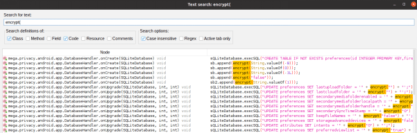
As with most Android applications, a good way to find out information about it is to decompile the application. I used Jadx 1.53 for this and the process seemed to work without any significant problems. I downloaded Threema-6.3.0-1113.apk to decompile.
It appears that the key.dat file is considered a version 1 key file with the master_key.dat file being version 2. The below fragment of code is taken from MasterKeyFileProvider.java:
    public final File getVersion2MasterKeyFile() {
        return new File(this.directory, "master_key.dat");
    }

    public final File getVersion1MasterKeyFile() {
        return new File(this.directory, "key.dat");
    }
Given that the version I had used the master_key.dat and that the version 1 file is covered by the Github code previously referenced, I’ll only be detailing the version 2 process.
It appears that the readKeyFile function from lines 36 – 44 of the Version2MasterKeyFileManager.java file shows the start of the process
public final MasterKeyStorageData readKeyFile() throws IllegalAccessException, IOException, IllegalArgumentException, InvocationTargetException { DataInputStream dataInputStream = new DataInputStream(new AtomicFile(this.keyFile).openRead()); try { MasterKeyStorageData.Version2 version2DecodeOuterKeyStorage = this.decoder.decodeOuterKeyStorage(dataInputStream); CloseableKt.closeFinally(dataInputStream, null); return version2DecodeOuterKeyStorage; } finally { } }
This takes us to Version2MasterKeyStorageDecoder.java at line 67
public final MasterKeyStorageData.Version2 decodeOuterKeyStorage(DataInputStream inputStream) throws IOException { Intrinsics.checkNotNullParameter(inputStream, "inputStream"); int unsignedShort = inputStream.readUnsignedShort(); OuterKeyStorage$Version outerKeyStorage$VersionForNumber = OuterKeyStorage$Version.forNumber(unsignedShort); if ((outerKeyStorage$VersionForNumber == null ? -1 : WhenMappings.$EnumSwitchMapping$0[outerKeyStorage$VersionForNumber.ordinal()]) == 1) { return decodeOuterKeyStorageV1(inputStream); } throw new IllegalStateException(("Unsupported outer version number " + unsignedShort).toString()); }
Breaking this down gives us:
int unsignedShort = inputStream.readUnsignedShort();
Reads the first 2 bytes of the file as an unsigned 16-bit integer(big-endian). This is the version number.
OuterKeyStorage$Version outerKeyStorage$VersionForNumber =
OuterKeyStorage$Version.forNumber(unsignedShort);
Converts the integer to an enum value. The code for this can be seen below:
OuterKeyStorage$Version.forNumber():public static OuterKeyStorage$Version forNumber(int value) {if (value != 0) {return null; // Unknown version}return V1_0; // Only version 0 is recognized}
This shows us that there is currently only a version 1 of this file format. If the first two bytes of your master_key.dat file are not 0x00 0x00 then it may have been updated since version 6.3. Assuming the version is 1, the decodeOuterKeyStorageV1 function is then called (line 77 of the same file):
public final MasterKeyStorageData.Version2 decodeOuterKeyStorageV1(DataInputStream dataInputStream) throws IllegalAccessException, IOException, IllegalArgumentException, InvocationTargetException { OuterKeyStorageV1 from = OuterKeyStorageV1.parseFrom(dataInputStream); if (from.hasArgon2IdProtectedIntermediate()) { OuterKeyStorageV1.Argon2idProtected argon2IdProtectedIntermediate = from.getArgon2IdProtectedIntermediate(); Intrinsics.checkNotNull(argon2IdProtectedIntermediate); byte[] byteArray = argon2IdProtectedIntermediate.getEncryptedIntermediate().toByteArray(); Intrinsics.checkNotNullExpressionValue(byteArray, "toByteArray(...)"); EncryptedDataAndNonce encryptedDataAndNonceSeparateEncryptedDataAndNonce = ProtobufExtensionsKt.separateEncryptedDataAndNonce(byteArray); OuterKeyStorageV1.Argon2idProtected.Argon2Version version = argon2IdProtectedIntermediate.getVersion(); if ((version == null ? -1 : WhenMappings.$EnumSwitchMapping$1[version.ordinal()]) == 1) { Argon2Version argon2Version = Argon2Version.VERSION_1_3; CryptographicByteArray cryptographicByteArray = ByteArrayExtensionsKt.toCryptographicByteArray(encryptedDataAndNonceSeparateEncryptedDataAndNonce.getData()); CryptographicByteArray cryptographicByteArray2 = ByteArrayExtensionsKt.toCryptographicByteArray(encryptedDataAndNonceSeparateEncryptedDataAndNonce.getNonce()); int memoryBytes = argon2IdProtectedIntermediate.getMemoryBytes(); ByteString salt = argon2IdProtectedIntermediate.getSalt(); Intrinsics.checkNotNullExpressionValue(salt, "getSalt(...)"); return new MasterKeyStorageData.Version2(new Version2MasterKeyStorageOuterData.PassphraseProtected(argon2Version, cryptographicByteArray, cryptographicByteArray2, memoryBytes, ch.threema.base.utils.ProtobufExtensionsKt.toCryptographicByteArray(salt), argon2IdProtectedIntermediate.getIterations(), argon2IdProtectedIntermediate.getParallelism())); } throw new IllegalStateException(("Unsupported argon2 version " + argon2IdProtectedIntermediate.getVersion()).toString()); } if (from.hasPlaintextIntermediate()) { ByteString plaintextIntermediate = from.getPlaintextIntermediate(); Intrinsics.checkNotNull(plaintextIntermediate); DataInputStream dataInputStream2 = new DataInputStream(plaintextIntermediate.newInput()); try { MasterKeyStorageData.Version2 version2 = new MasterKeyStorageData.Version2(new Version2MasterKeyStorageOuterData.NotPassphraseProtected(decodeIntermediateKeyStorage(dataInputStream2))); CloseableKt.closeFinally(dataInputStream2, null); return version2; } finally { } } else { throw new IllegalStateException("Invalid outer key storage"); } }
This code is a bit more complicated, but it basically boils down to:
The master_key.dat file is a protobuf file
Checks if protobuf field 2 (argon2id_protected_intermediate) is present. This
means the key is passphrase-protected.
If true, gets the Argon2idProtected sub-message containing:
version (Argon2 version)
salt (random bytes)
memory_bytes, iterations, parallelism (Argon2 parameters)
If not, checks if protobuf field 1 (plaintext_intermediate) is present. This means no
passphrase protection at the outer layer. (This was the case with my file)
As my file was a plaintext_intermediate, I can only demonstrate this at this time. Maybe in the future I can test against a argon2id_protected_intermediate version.
The following functions get called from here which aren’t described in any detail:
decodeIntermediateKeyStorage ──►
decodeIntermediateKeyStorageV1 ──►
decodeInnerKeyStorageV1 ──►
Version2MasterKeyStorageInnerData
The final function ends us with this function:
    public final Version2MasterKeyStorageInnerData.Unprotected decodeInnerKeyStorageV1(DataInputStream dataInputStream) {
        byte[] byteArray = InnerKeyStorageV1.parseFrom(dataInputStream).getMasterKey().toByteArray();
        Intrinsics.checkNotNullExpressionValue(byteArray, "toByteArray(...)");
        return new Version2MasterKeyStorageInnerData.Unprotected(new MasterKeyData(byteArray));
    }
InnerKeyStorageV1.parseFrom(dataInputStream).getMasterKey().toByteArray();
This does three things in one line:
Parses protobuf message
Gets the master_key field (ByteString)
Converts to raw byte[]
The InnerKeyStorageV1 protobuf structure is simple:
message InnerKeyStorageV1 {
bytes master_key = 1; // The actual 32-byte master key
}
This tells us that, if plaintext_intermediate is being used, that the 32 byte encryption key is stored as raw bytes in the file. I used the https://protobuf-decoder.netlify.app/ website to take the hex values of my file and then decode the protobuf. As you can see in the example below, the last field contains my encryption key. To get the hex values of my file i used the command below, which is a linux command, but you could easily export the hex as text from WinHex or a similar tool
xxd -p master_key.dat | tr -d '\n'
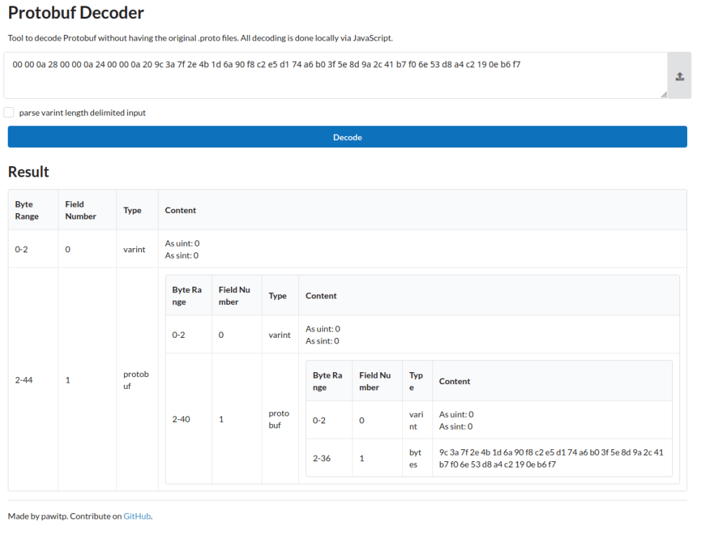
This now gives us a key and for the purpose of this example I will use a random example:9c3a7f2e4b1d6a90f8c2e5d174a6b03f5e8d9a2c41b7f06e53d8a4c2190eb6f7
Now that we have a key, we need to determine the parameters required to decrypt the database. In the issues from the Github project mentioned before, some settings are specified:
PRAGMA cipher_default_kdf_iter = 1;PRAGMA key='$key';PRAGMA kdf_iter = 1;PRAGMA cipher_memory_security = OFF;
However its always best to verify this in the code and this can be found in DatabaseService.java lines 124-135:
  new SQLiteDatabaseHook() {
      public void preKey(SQLiteConnection connection) {
          connection.executeForString("PRAGMA cipher_log_level = NONE;", ...);
          connection.execute("PRAGMA cipher_default_kdf_iter = 1;", ...);
      }

      public void postKey(SQLiteConnection connection) {
          connection.execute("PRAGMA kdf_iter = 1;", ...);
      }
  }
Aside from the “PRAGMA cipher_memory_security = OFF;”, all of the settings can be seen here. With this verified, we can use sqlcipher to decode the database:
sqlcipher threema4.db "PRAGMA cipher_default_kdf_iter = 1; PRAGMA key = 'x\"9c3a7f2e4b1d6a90f8c2e5d174a6b03f5e8d9a2c41b7f06e53d8a4c2190eb6f7\"'; PRAGMA kdf_iter = 1; SELECT * FROM sqlite_master;"
Here the threema4.db is passed to sqlcipher, along with the required key and PRAGMA statements, and then executing the SQL query “Select * from SQLITE_MASTER” which is the table that contains the details of all the tables in the database. This should provide you with output similar to:
table|contacts|contacts|2|CREATE TABLE contacts (identity VARCHAR........
However it’s much easier to work with a decrypted database and this command can be used to convert the database to its unencrypted form:
sqlcipher threema4.db "PRAGMA cipher_default_kdf_iter = 1; PRAGMA key = 'x\"9c3a7f2e4b1d6a90f8c2e5d174a6b03f5e8d9a2c41b7f06e53d8a4c2190eb6f7\"'; PRAGMA kdf_iter = 1; ATTACH DATABASE 'threema4_decrypted.db' AS plaintext KEY ''; SELECT sqlcipher_export('plaintext'); DETACH DATABASE plaintext;"
Once this has been done, you can use a simple SQL query to recreate the messages and link them to the contacts
Select datetime(m.createdAtUtc/1000, "unixepoch") as CreatedTimeUTC, c.identity, c.publicnickname, m.body, m.state from message as mleft join contacts as con m.identity = c.identity
There are many other fields that exist within the tables that you might want to include, however this should give a good starting point. The query was tested and matched the messages as they were displayed on the app on the mobile device, it should be noted that times are stored in UTC so you may have to translate if your timezone is not GMT.